Importing Data
Houdini makes importing CSVs and their specific data simple with the table import SOP. Before jumping right into it, it’s worth taking a brief look at the table and how its data are structured.
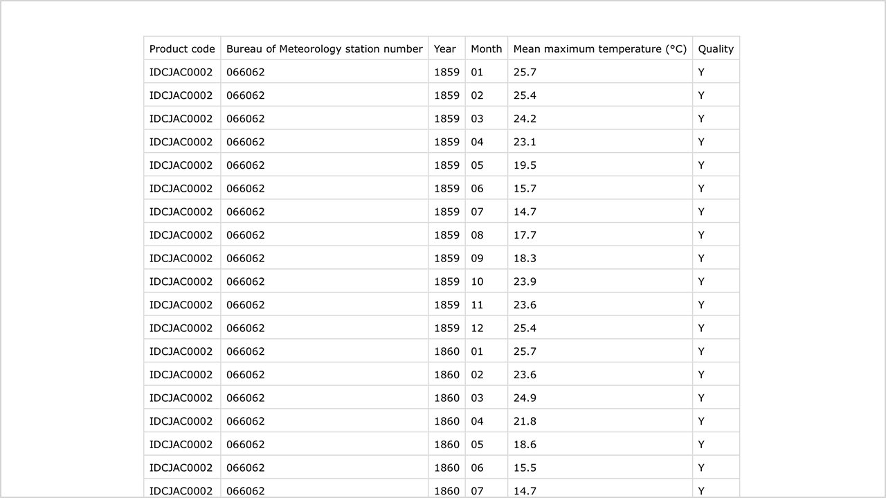

Spreadsheet structure
From this very basic table, we’re just interested in year, month and temperature data. As column counting begins at index 0, we’re therefore looking at columns 2, 3, and 4. We’ll just work with the first year to start which will be the first 12 rows. Head back into Houdini and drop a table import SOP into the network and make sure that geometry spreadsheet pane is still open. Load the CSV into the node through the file parameter and create an attribute called “temp” which we’ll use to store incoming temperature data. Looking back at the spreadsheet we’ll need to set our column number to 4 to receive the correct data. Keep the type as a float as we’re dealing with numbers with decimals, and we only have one kind of temperature data so attribute length should sit at 1.
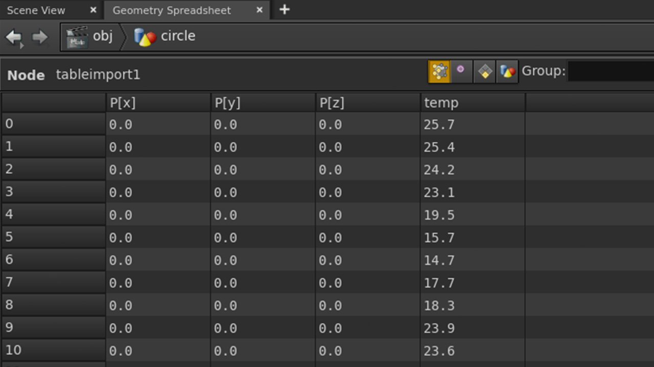

Geometry spreadsheet, points view, table import selected
With the table import node selected, have another look under points in the geometry spreadsheet and you’ll see our new temp attribute storing our data. As mentioned, we only want to work with one year first, so set “max rows” to 12. Referencing data from the spreadsheet isn’t as straightforward as connecting the table import node to our geometry. In fact, the table import node doesn’t need to be connected at all and can stay by itself in the network view. We’ll be connecting to its data via an expression.
The original nodes we created worked off the base circle shape and left us with 12 primitives, which is exactly what we want to match our month-oriented dataset. Coming off this (and we’ll have to remove that connection to the sweep node for a moment), we need to add an attribute create SOP. We need to create a new primitive attribute that reads from our CSV, using the input primitive data as a reference. In other words, we’ll match the first primitive of our segmented circle to the month of January, and so forth. Add an attribute create sop to our resample node, and we’ll give it a name of “t” for temperature and a class of primitive. The only other parameter we need to complete is value. Houdini is asking us, “what are we writing into this attribute?”
We want to pull data from the table import SOP, which is outputting as points, so we’ll need to access it with the point() expression function. Have a look at the documentation for point. We’ll need to provide a few things: the surface node (our table import), the point number (we’ll use our inputting primitive numbers), attribute (our original attribute name) and index (where in this attribute are we looking?).
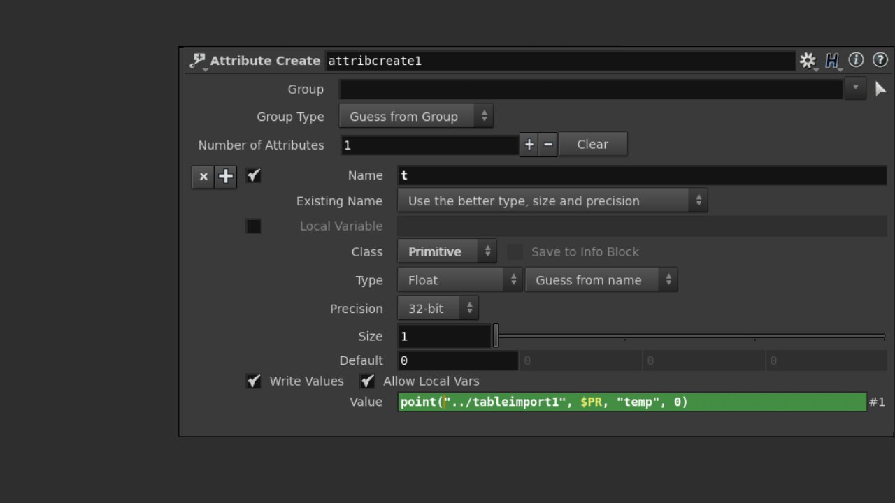

Create attribute node parameters
We reference our table import node like a file in a directory, so we step out from the attribute create node first then into the table node via “../tableimport1”. The point number isn’t a single value because we have multiple primitives, so using the variable $PR will access each and every inputting primitive and add it to our new attribute t. The original attribute name we chose was temp, and when we made this attribute we only gave it the length of one value so it’s at index 0.
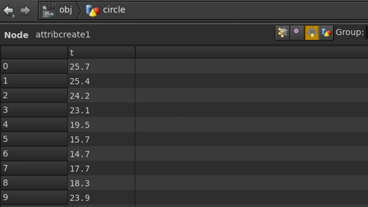

Geometry spreadsheet, primitives view, attribute create selected
Now check the primitives section of our geo spreadsheet and find the first 12 months of weather data stored as primitives. Great! The only problem is that our actual 3D shapes are drawn from points (remember sweep?), so we’re going to need to convert this attribute back into points. You might be wondering why this is as table import was delivering points anyway. While true, we need attribute create to assign the correct values to each primitive. If we don’t, we might end up with different temperature values assigned to points of the same segment. To fix this we have to grab data from our CSV, assign it to the correct primitive, then promote our geometry into points so that the two or four or forty points per primitive are all reading off the same month.
Connect the output of our attribute create node to an attribute promote SOP. Keep the original name of “t” and let’s promote from our original class of primitive to a new class of point. Now we should select this new node and check the geometry spreadsheet under points. Try adjusting the maximum segments value (resample node) again and notice that while each primitive might have tens of points, each is equal to the same value.
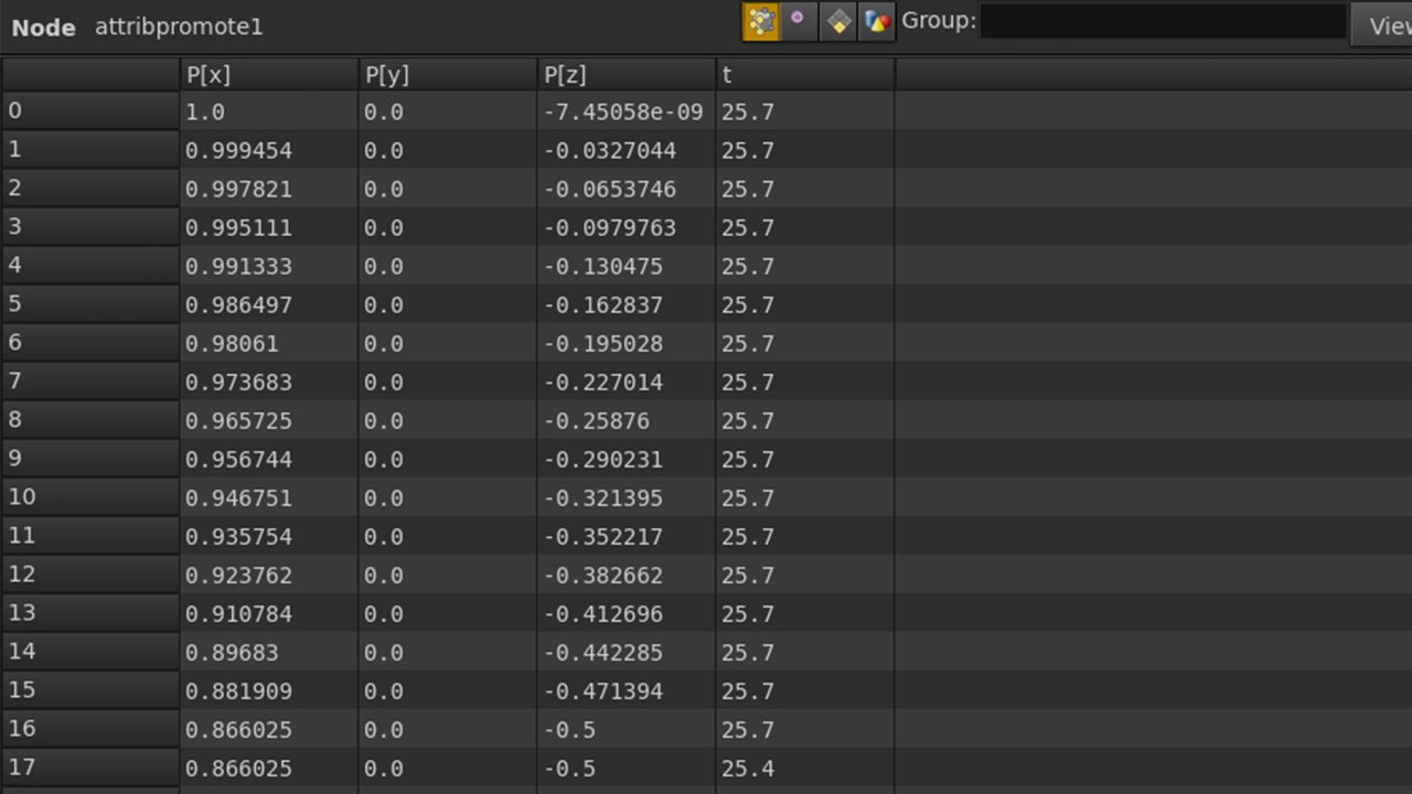

Geometry spreadsheet, points view, attribute promote selected
Now we have a number “t” assigned to every single point in our geometry, so we can move on to work with colour. Houdini has a few ways to add colour, but rather than just using the value of “t” to assign a brightness or level of red, we can access a point in a divergent colour scheme that progresses from blue to white to red. To do this, we’ll need to use a point wrangle SOP, a very powerful node that lets you modify attributes point by point. In this case, we’ll run over all points in our geometry and assign a colour to them using the @Cd attribute.
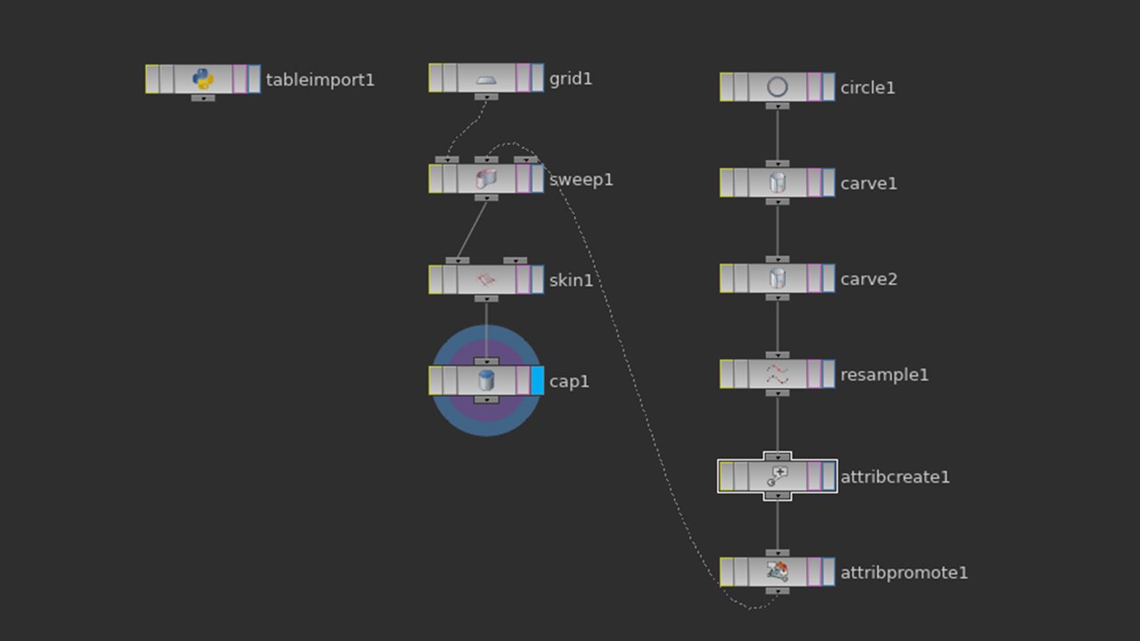

Current network view
Add a point wrangle node to your network, and make sure it runs over points (this will sit in between our attribute promote and sweep nodes). We’ll need to write a snippet of VEX code to make this work. Here is some that was prepared earlier.
vector col_values[] = {
    {103,0,31},
    {178,24,43},
    {214,96,77},
    {244,165,130},
    {253,219,199},
    {240, 230, 255},
    {170, 170, 210},
    {120,120,170},
    {90,90,130},
    {40,40,80},
    {0,0,40}
};

int i = int( fit(@t, 13.4, 29.5, 10, 0) );
@Cd = col_values[i] / 255;
Let’s break this down. The first block is an array of RGB values, so each set of three values is a single colour. There are ten colours here in total. The next line establishes a variable “i” which uses the fit() function to re-map our temperatures ranging from 13.4–29.5ºc into the scale of 0–10 which is our colour range. Once we have that number, we find where it lies in our array of colours and then assign it to @Cd which is an already known attribute for the point’s colour.
Now we can connect the output of our point wrangle node to the second input of sweep.
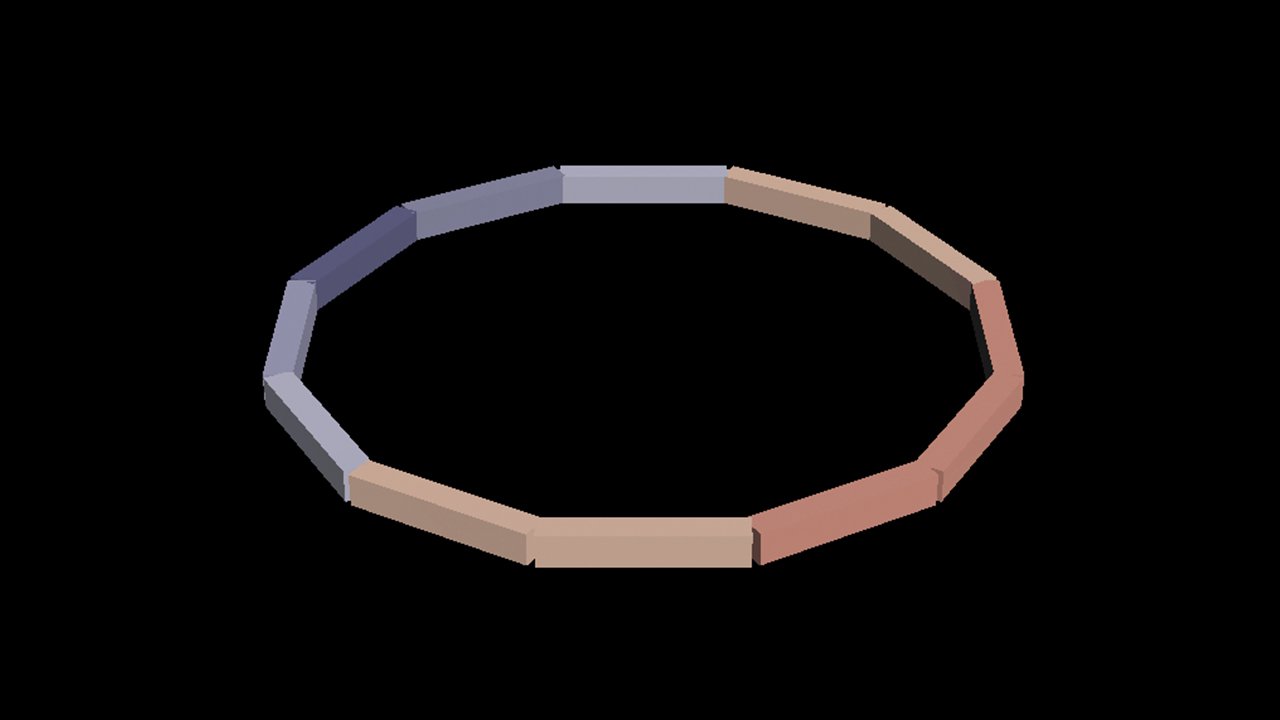

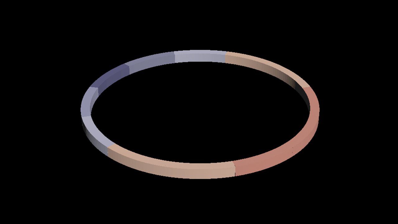

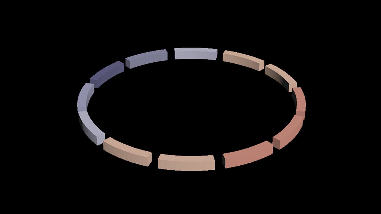

Variations in segment length and carve settings